What is the Substitution Effect in Economics?

Relative price changes are the catalyst for the substitution effect. When faced with a price change of one good relative to a related good, consumers typically seek to maximize their utility (i.e., satisfaction) from adjusting their consumption choices. They will tend to substitute extra consumption of the relatively cheaper good in place of the relatively more expensive good.

This adjustment occurs while holding the total level of satisfaction (i.e., utility) constant.

Note that I pointed out that the substitution effect applies between related goods. For example, if the price of coffee increases while tea stays the same, it is likely that consumers will substitute more tea for less coffee. However, a rise in the price of coffee is unlikely to have any direct substitution effect on the demand for crude oil, cinema tickets, football boots, or any other types of unrelated products.

Nevertheless, since incomes are constrained, any increase in expenditure on one good must necessarily also have an impact on other goods, related or not.

Factors Influencing the Substitution Effect

The strength of the substitution effect can vary depending on several factors. One crucial factor is the availability and accessibility of substitute products. If there are numerous substitute products readily available in the market, consumers are more likely to switch to a lower-priced alternative when the price of a particular product increases.

The level of brand loyalty to a given product can also impact the strength of the substitution effect. If a consumer has a strong attachment to a particular brand or product, they may be less likely to switch to a substitute, even if the price is significantly lower.

Timeframe is also an important consideration because consumers do not immediately adjust their spending patterns when the price of certain goods change. For some goods, prices are very responsive in the short-term, but for other goods it takes more time to adjust. See the real world examples below for more information on this.

Substitution Effect Graph

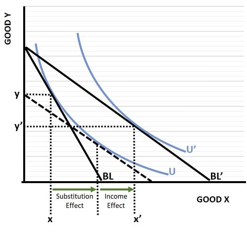
In the substitution effect graph below, I have illustrated how a consumer changes his/her preferred combinations of goods x and y. For an explanation of how this graph works, you can read my articles about the Budget Line and the Indifference Curve.

The initial preferred bundle of goods occurs where the highest possible indifference curve (U) just touches the budget line (BL). At this point, the consumer purchases x,y amounts as indicated by the dotted lines.

Now, after the price of good x falls, the consumer purchases much more of it, and actually reduces consumption of good y in order to be able to further increase consumption of good x. The new preferred consumption bundle occurs at x',y'.

There are two effects at work here, one is the substitution effect and the other is called the income effect.

Substitution Effect vs. Income Effect

The substitution effect tends to work in conjunction with the income effect, because when the price of one product changes relative to a related product, it will affect total purchasing power of a given income (or budget constraint).

For example, when the price of coffee falls, consumers will tend to consume more of it instead of alternative beverages, but they may also have some spare income remaining that can be spent on other goods & services. For more details about this, see my article:

• What is The Income Effect in Economics?

The extent to which each effect dominates the other depends entirely on the nature of the good itself. For details on this, see my article about Types of Economic Goods, and especially about Complementary Goods & Substitute Goods

Real-World Examples of Substitution Effects

The substitution effect is not merely an abstract concept in economics; it has real-world implications and applications that affect both individual consumers and entire markets. Here are some practical examples of how the substitution effect manifests in various economic scenarios.

• Consumer Goods – In highly competitive markets where consumers have many similar products to choose from, the substitution effect will tend to be larger. For example, when the price of a particular smartphone model drops significantly, consumers may shift their preferences and purchase the more affordable options, substituting them for the more expensive product.
• Energy Sources – In the energy sector, the substitution effect plays a limited role in shaping energy consumption patterns in the short-run. When the price of gasoline rises, consumers may reduce their driving and opt for public transportation or carpooling as a means of substitution. Over the long-term, consumers will tend to substitute more fuel-efficient cars e.g., with smaller engines, or go for hybrids and electric cars instead.
• Labor Market – The labor market is not immune to the substitution effect. As wages for certain professions rise or fall, employers may prefer to offer fewer/extra hours of work each week. As with the gasoline example, the substitution effect here will be larger in the long-run because employers will be able to switch their production techniques towards a more labor-intensive method, or a more labor-saving technique, given enough time. They do this in order to minimize their costs of production.

Limitations and Criticisms

While the substitution effect is a valuable tool for analyzing consumer behavior and market dynamics, it is not without its limitations and criticisms. The following limitations and criticisms are applicable:

• Simplistic Assumptions – The concept relies on the assumption of rational consumer behavior, and measuring it requires constant utility. In reality, consumer decisions are influenced by a multitude of factors, including emotions, habits, and social influences, which may not align with these conditions.
• Neglects Other Factors – It isolates the impact of relative price changes while holding income constant. However, in the real world, changes in income and prices often occur simultaneously, thereby making it difficult to make reliable calculations.

Related Pages:

• The Income Effect
• Consumer Behavior
• Revealed Preference
• The Engel Curve
• The Price Consumption Curve

ShareFacebookXPinterestTumblrRedditWhatsApp