- Home
- Aggregate Demand
- Keynesian Multiplier

The Keynesian Multiplier
As a concept in economics, the Keynesian multiplier is very straight forward and not at all controversial. Where disagreement might surface relates more to its size, or rather what size is desirable, and what the correct macroeconomic policy is to achieve that size.
For illustrative purposes I'll be using the model that was developed on my page about:
In order to reduce repetition, it would be best to start with that page unless you already understand how the consumption function model works.
A reduction in the Multiplier
There are a multitude of ways in which an economic policy mix will affect the Keynesian multiplier, but lets start with the most obvious example i.e. a tax increase.
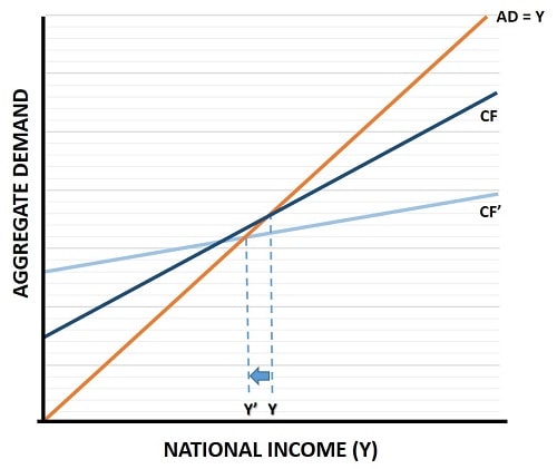
In the graph below, the dark blue consumption function (CF) represents a theoretical world with no government or foreign trade, and where all goods & services are produced by the private sector.

In this world the multiplier will be very strong, and anything that causes a shift in CF (such as an increase in Investment due to better business confidence levels) will cause a proportionate shift in aggregate demand, but a much larger shift in national income. I'll demonstrate this below, but for now lets just take that for granted.
Now, for whatever reason, society decides that some goods and services would be better provided by a government instead of a private market and so it decides to levy a tax on citizens in order to pay for those goods and services.
The impact of this is to disassociate those government provided goods and services from national income. Of course, these things can't be disassociated forever, but for a short time we can regard them that way because governments can borrow money when national income is low in order to continue providing these products.
After the government puts the tax and spend policy in place, the slope of the consumption function will change and become less steep. CF' in the graph represents this change and you'll notice that at low levels of national income aggregate demand is higher and, conversely, lower at high levels of income. This happens due to the effect of increased government borrowing (to support the economy) when income is low, and increased tax receipts when income is high (which slows the economy down). E.g. an income tax raised as a proportion of income will result in higher taxes when income is higher, allowing a surplus (or at least a reduced deficit) to develop.
A more interesting point to note, and slightly controversial point, relates to the impact on national income once the government tax and spend policy is introduced. I have illustrated in the graph a slight reduction in national income from Y to Y' as a consequence of the policy. The reason for this is that there will be some loss of efficiency implied by the policy. This is not a criticism of the policy in and of itself, it is just a cost of gaining some extra stability in the economy.
There are, of course, some products (called public goods) that the private sector cannot provide in an efficient manner and that the government can do a better job of providing. For these public goods you could draw a new CF that gives society both more stability and a higher national income. There are also some government taxes and subsidies that work to correct market failures, and these too can increase national income and stability.
However, with these sorts of exceptions noted, the total weight of evidence is clear, and that is that governments operate with less efficiency than competitive markets, and so we have to accept some overall cost to national income as governments pay for their activities by taxing the private sector.
Later on I'll discuss a range of factors that cause changes to the size of the Keynesian multiplier, but first I want to demonstrate how the flatter CF' line gives greater economic stability.
How income tax affects the Keynesian Multiplier
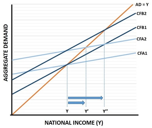
In the graph below I've illustrated the comparative volatility of national income before and after the government income tax is introduced. The CFB1 line shows the starting consumption function before the income tax comes into force. CFA1 shows the situation after the tax is adopted.
For simplicity lets pretend that there is no initial affect on the level of national income from efficiency losses, and that national income holds steady at a level of Y.
Now, after an increase in one of the autonomous components of aggregate demand (again - see my article about the consumption function if that doesn't make sense), we can see what would happen to national income in an economy with income taxes and one without.

The CFB2 line now intercepts the AD=Y line at a national income of Y'', showing a huge increase in income in an economy before any income tax policy is adopted.
However, the same increase in aggregate demand in an economy after the income tax policy is adopted yields a much smaller increase in national income to Y'.
At this point you might be thinking that this is one more reason to hate income taxes, but think about it a little longer. Autonomous increases in aggregate demand are a fine thing, but what about autonomous decreases? In that event the reverse process would yield much deeper cuts to national income in an economy with no income taxes.
This is the point, income volatility i.e. severe booms and recessions, is reduced by the income tax policy because as an economy grows and income rises, more taxes are drawn out of the economy automatically, and this helps prevent overheating in the economy. Similarly, when downturns occur, less money is paid in income tax and so the decline is softened and less severe.
In the jargon of the Keynesian multiplier, you can see that there is a multiplied impact on the economy from shifts in aggregate demand when there are no income taxes. This is the meaning of the Keynesian multiplier - it relates to the relative size of change in national income compared to the size of the aggregate demand shift that caused it.
But what causes the Keynesian Multiplier?
Let's start again from the beginning with a simple economy with no government or foreign trade where all output is produced by the private sector free-market.
Now, suppose that you start a new job that pays you an extra $100 dollars more than your old job. Suppose also that your own personal marginal propensity to consume (MPC) is 0.8 meaning that you will spend 80% of your extra income and save the other 20%.
Initially that extra spending will cause aggregate demand to rise by $80, but this is just the start. When you spend that $80, someone else receives it as an increase in their income. For example suppose you bought some new shoes, the shoe salesman now has an extra $80 and, assuming for simplicity that his MPC is also 0.8, he will spend an extra $64 and save the remaining $16. If he spends this at a restaurant then the restaurateur makes an extra $64 which increases his spending and so on.
At the end of this process, the multiplied effect on the economy will work out as an increase in demand of $500. How do we know - because in this simple economy the formula for calculating the multiplier is 1/MPC, or 1/0.2, which equals 5. So the initial $100 increases national income by a multiplier of 5 which gives $500.
Factors that reduce the Multiplier
You can probably guess that there are many more factors than just income taxes that reduce the Keynesian multiplier. All taxes have a part in reducing it since they all reduce disposable income, but some taxes have more effect than others.
Marginal taxes i.e. those that apply to the increase in income rather than general income have the biggest affect. Flat rate taxes have the least effect, expenditure taxes like V.A.T. sit somewhere in between.
The government welfare state also reduces the multiplier because the reduction in consumer spending is lessened when unemployed people have access to state support.
Foreign trade also reduces the multiplier because, as national income rises, any increase in spending will go in part towards imported products rather than domestic products.
The economy's capacity to increase output is also clearly a factor that effects the multiplier, and whilst the Keynesians tend to assume plenty of spare capacity to raise output as required, the reality is that there is usually some trade-off between increased output and a higher price level.
A major limiting factor to the multiplier occurs when consumer spending fails to increase as a result of an increase in disposable income e.g. from a temporary tax cut (or an increase in stimulus checks) because consumers simply save the extra money or use it to pay off credit card debts and personal loans. These temporary, or 'transitory' changes in income are known to be less effective at boosting spending, and for more information on that, see my article:
The National debt and the budget deficit also need to be included on the list of factors that reduce the multiplier. Servicing the debt is a costly and significant drain on resources such that extra taxes or extra borrowing must be incurred. If extra taxes are raised, disposable income is reduced and therefore the multiplier is reduced directly. If extra borrowing is incurred then, all else equal, interest rates will start to rise and cause a monetary contraction which will depress any growth in the economy.
Keynesian Multiplier Estimate
Prior to the quantitative easing following the 2008 financial meltdown, the multiplier was probably somewhere in the region of 1.4 to 1.6 most of the time.
In modern times the multiplier has been shrinking to ever lower levels as the national debt has climbed ever higher. These days it is hard to argue that there is any multiplied effect at all on national income arising form spending increases, so the Keynesian multiplier is probably somewhere close to unity.
Sources:
Related Pages: