The Inverse Demand Function (Formula, Graph, & Example)

The concept of an inverse demand function, and its mathematical expression, is derived from Alfred Marshall’s original work on demand in his book, Principles of Economics (1890). While Marshall did not explicitly separate inverse demand functions as a distinct concept, his work laid the foundation for their later development and application in economic theory.

The inverse demand function expresses the price (P) of a good as a function of the quantity demanded (Q), typically written as P=f(Q). In contrast to the standard demand function, which relates quantity demanded to price Q=f(P), the inverse demand function shows how much consumers are willing to pay for a given quantity of a good.

As you can imagine, this information is not really relevant for small producers in competitive markets, because those producers are ‘price takers’ i.e., no matter what quantity they produce it is only a small part of overall production and has no influence on the market price. However, producers in less competitive industries do have influence on price, and so they are interested in formulating this.

Economists and other market analysts are also interested in modeling entire industries, and the inverse demand function is commonly used in microeconomics for this purpose. It is primarily used to:

• Calculate the market-clearing price for a given quantity of goods.
• Analyze the marginal revenue for a monopolist, as the derivative of the inverse demand function gives the marginal revenue function.
• Evaluate consumer surplus, producer surplus, and deadweight loss in market equilibrium.
• Assist firms in deciding optimal pricing strategies and output levels.

Inverse Demand Function Formula

The standard Marshallian demand function, as noted above, takes the form Q=f(P), and this is typically simplified to the standard linear demand function Qd = a – bP where:

• Qd = the quantity of a good demanded
• a = the maximum amount demanded i.e., when price is zero.
• b = the responsiveness if demand to price changes
• P = price

The inverse demand function formula then rearranges this formula via a simple mathematical transposition to focus of price i.e.:

P = (a – Qd)/b

This is the inverse demand function formula for a simple straight line linear demand curve. The same process is used to transpose more complex functions, but the simple function above is most commonly used for simplicity.

Inverse Demand Function Graph

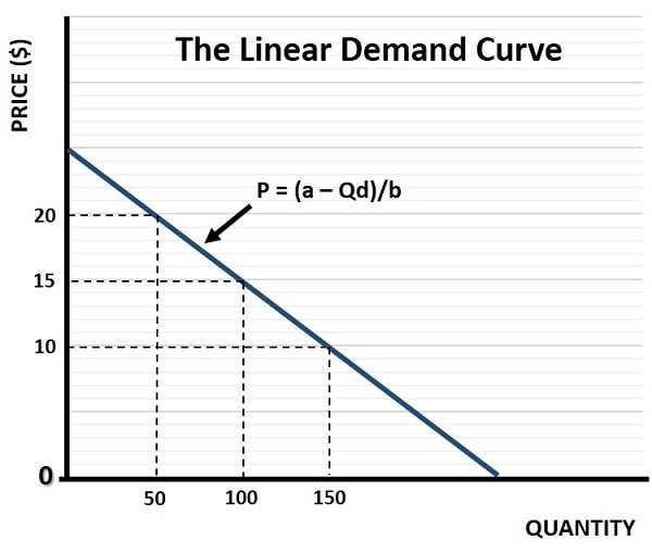
An inverse demand graph is identical to a normal demand curve, and is illustrated below:

I’ve again used a linear inverse demand curve as it simplifies calculations, but technically a normal demand curve is not linear, it is curved. For the reasons why, click the link, but we needn’t worry about this here as it doesn’t change the important points about the inverse demand function.

Inverse Demand Function Example

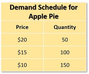
Calculating inverse demand from a demand schedule is simple if we stick with the linear demand model above. All we need to do is solve the equation of a straight line, which is a simple mathematical problem from our school days. As an example, consider the following demand schedule for daily apple pies in a local town:

Using the inverse demand function P = (a – Qd)/b we can start by solving the slope (b) by calculating the change in quantity divided by the change in price as we move from two price/quantity points. So, if we move from $20 to $15, we also move from a quantity of 50 apple pies to 100 apple pies. That’s a change of 50 apple pies and $5. So, the slope of this linear curve is 50/5 i.e., 10. Technically the slope is -10, but we use the positive value since our linear demand curve Qd = a – bP already has a negative, and a double negative would become a positive which defies the first rule of demand i.e., that the demand curve is downward sloping.

Next, we solve for demand when price is zero, which gives us (a). Since the schedule tells us that demand is 150 when price is $10, and we know that the slope of the curve (b) is 10, we know that a $10 reduction in price (to $0) would lead to a 10x10 increase in quantity (to 250). So, (a) is equal to 250.

Substituting these values into the inverse demand function P = (a – Qd)/b we get:

P = (250 – Qd)/10

This is the inverse demand function for this simple linear demand curve, and we can verify by checking what the quantity demanded would be when the price is $15:

15 = (250 – Qd)/10

150 = 250 – Qd

Qd + 150 = 250

Qd = 100

QED this is as indicated by the demand schedule. The point is that we can now use the same function to calculate what the quantity would be at prices not shown in the schedule, which is very useful information for any economic agent that wishes to model the apple pie industry in this particular local town.

Weaknesses

The weaknesses of the basic inverse demand function relate mostly to the other forces that affect the market but that are not included. These do not really compromise the function, and more complex functions can be devised to account for most of the weaknesses. However, it helps to remind ourselves of some important considerations when using such functions. They:

• Assume other factors (e.g., income, preferences) remain constant, which may not reflect real-world complexity.
• May oversimplify demand relationships by ignoring cross-elasticities and substitution effects.
• Rely on accurate data to estimate the function, which can be difficult to obtain.

As an additional reminder, inverse demand functions focus on entire markets and are therefore of most use to firms that dominate entire markets. In highly competitive markets, the focus is typically on supply rather than firm-specific demand functions.

FAQs about the Inverse Demand Function

Related Pages:

• The Compensated Demand Function
• Derived Demand
• Consumer Surplus
• Elasticity of Demand
• Consumer Behavior

ShareFacebookXPinterestTumblrRedditWhatsApp