The Demand Curve in Economics (Types, Slope, Shifts, & Examples)

The demand curve in economics is one of the first concepts that students of microeconomics are introduced to. It represents the relationship between the price of a good or service and the associated quantity demanded of it by consumers over a given period.

The concept of demand is rooted in the work of Alfred Marshall, a British economist. In his book, Principles of Economics (1890), Marshall formalized the relationship between price and quantity through demand and supply curves. He introduced the idea of demand curves as downward-sloping and emphasized their use in economic analysis.

The first law of demand states that (with all other factors held constant) as the price of a product increases, less of it will be demanded. The same logic applies for a price decrease i.e. it will lead to an increase in demand. This law is a general law that applies in the vast majority cases, but there are some exceptions as described in my article about: Types of Economics Goods

The first law of demand gives rise to the downward sloping demand curve that is so commonly depicted in economics text books, and the nature of that downward slope depends on many factors, the most important of which will be described below. Before getting into that, we should start with an explanation of individual demand, and then progress to a basic market demand curve using a demand schedule.

The Individual Demand Curve

Individual demand is simply the demand for a product that comes from one particular consumer. We do not typically draw a demand curve for any single consumer because we usually draw demand curves for an entire market, and we usually assume that there will be many buyers in a market.

This is certainly the case in a competitive market, but we should keep in mind that there are cases where a single buyer (or a small number of buyers) can dominate a market. This type of market would be called a monopsonist market, but I will continue here with the assumption of many buyers.

An individual consumer will likely wish to consume more of a product as its price falls simply because we assume that more consumption is better than less consumption. It may be that there is a limit to how much pizza a consumer wishes to consume in any given period, but such extremes are rarely visited in practice because there is an almost unlimited array of competing products that we also wish to consume, and we only have limited resources with which to purchase them.

Each product competes with all the other available products for our custom, and we maximize our total well-being (economists call this ‘utility’) by allocating our finite incomes across many different products according to our specific preferences. We will, therefore, choose to consume only so much pizza, at any given price, until we prefer to spend our money on something else. However, if that given price were to fall, we would then tend to prefer more pizza, and so on.

In essence, there are two underlying forces that support the first law of demand:

• The Income Effect – A price decrease effectively increases consumers’ purchasing power. This allows them to buy more of the good, increasing quantity demanded.
• The Substitution Effect – When the price of a certain good falls, it becomes relatively cheaper compared to alternatives (substitutes). Consumers will likely switch more spending in favor of it, and away from those relatively more expensive substitute goods.

The Market Demand Curve & Demand Schedule

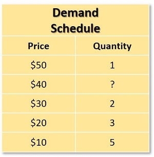
The market demand curve for a product is simply the sum of all individual demand curves for that product added together. Economists use a ‘demand schedule’ (presented in the form of a table) to represent all the relevant price and quantity combinations in the market. An example of this is given below:

Imagine that the demand schedule above relates to the price of your favorite pizza at a local restaurant. At $50 per pizza you might feel that the price is too high for regular consumption and therefore restrict yourself to one per month as a treat. If the price were on $10 per pizza, then you would happily increase consumption to five pizzas per month.

In between these prices the data is given for some more price output combinations, but the data is incomplete. Small gaps in data can easily be estimated from the general shape of the demand curve, for example, it’s easy to estimate that when the price is $40 there will be a quantity demanded between 1 and 2 pizzas per month. A process called ‘revealed preference’ can actually do quite a lot to estimate the whole market demand curve for all customers using very limited amounts of data.

The restaurant owner would like to construct a schedule of the type above for all his/her customers in order to know how his business sales would be affected at various price points. This information would allow the optimal price point to be chosen that would maximize profits.

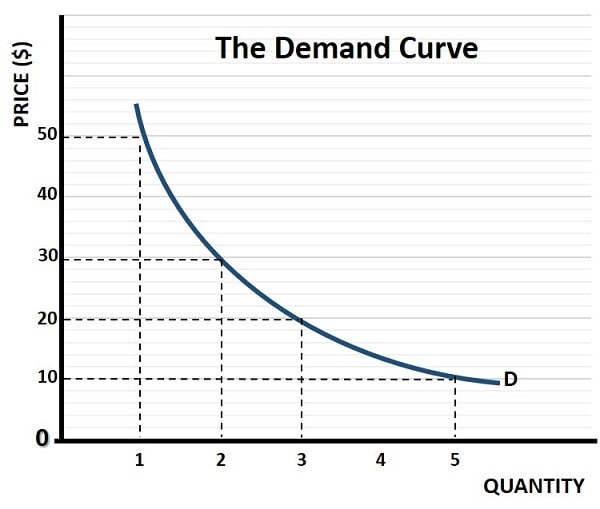
With a representative sample of information, rather than complete information (which cannot be obtained), the restaurant owner will be able to get an idea of the market demand curve for his pizzas. This is illustrated in the demand curve graph below.

As can be seen, the demand curve is downward sloping as predicted by the first law of demand i.e., that a higher quantity is demanded at lower prices. The second thing to notice is that the curve is bowed inwards (called convex to the origin) which displays a concept known as diminishing marginal utility. In a nutshell this means that the extra satisfaction gained from an additional unit of consumption falls as the overall level of consumption increases.

With a little reflection it should be obvious why this is the case; our enjoyment of a pizza (and all normal goods) is at its highest when it is relatively scarce. If we had pizza three times per day, we would likely grow sick of it very quickly, but at only one pizza per month we enjoy it so much that we will happily pay a high price to get it. For a fuller explanation of this important concept, have a read of my article at: Marginal Utility

I should also mention here that it is very common to see a simplified version of the market demand curve in the economics textbooks. Instead of the bowed demand curve shown on this page, economists tend to use a straight-line demand curve.

I’ve seen many commentators raise objections to the term ‘curve’ when what they see is actually a straight-line representation of demand, but economists use it for good reasons. It is known as the linear demand curve, and I advise you to click the link to see why it is so popular.

The Determinants of Demand

A common way to express the demand curve is via the function Qd = Qd(P). In words this simply means that the quantity demanded (Qd) is a function of price. Remember here that we continue to assume that all other influences are held constant, and only price is allowed to vary. This ensures that a single demand curve exists, and changes in price lead to a movement along that curve.

There are, of course, many other factors than price alone that determine the demand for a product. The most important of these are listed below:

• Income – when incomes are higher, consumers will tend to increase their demand for all sorts of goods and services.
• The price of related goods. These can be subdivided into two types: 1. Substitutes i.e., alternative products that compete with a good. 2. Compliments i.e., goods that are bought together with another good.
• Tastes and Preferences – these can be influenced by advertising, branding, fashions, trends, cultural influences and so on.
• Expectations – when consumers expect prices and/or quality levels to change in the future, this can cause current demand to change.
• Demographics – when more consumers enter a market, demand will increase and vice versa when the number of consumers decreases.
• Government regulations – regulations may prohibit or promote consumption, thereby affecting demand in the market.
• Seasonal forces – some products have higher demand at certain times of the year e.g. ice cream in summer, or skiing vacations during the winter.

Change in Demand Vs Change in Quantity Demanded

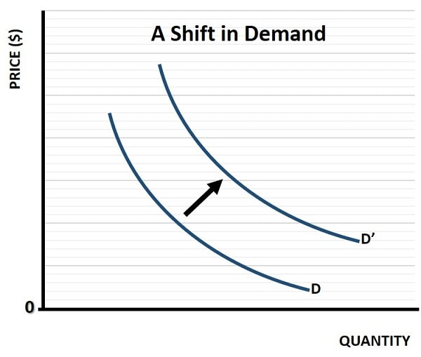
A demand shift vs movement along a demand curve occurs whenever one of the non-price determinants of demand (see list above) changes. As already noted above, changes in price result in a movement along an existing demand curve, but when a determinant other than price changes, a whole new curve is created. This is called a shift in demand, and is illustrated in the graph below:

Demand shifts can, of course, result in a rightward increase in demand (as in the graph above) or in a leftward decrease in demand, depending on circumstances. Sticking with the restaurant pizza example above, a shift in demand to the right could occur because the price of a competing product goes up (e.g. if Mexican restaurants became more expensive) which leads consumers to substitute more pizza instead.

Similarly, in the unlikely event that a new medical study was to prove beyond doubt that eating pizza every day would extend lifespan by 10 years then you can imagine that demand will increase exponentially. If that study went the other way and showed a decrease in lifespan then demand would collapse. These shifts in demand would occur at each and every price point, and it is this that creates a new demand curve. When price alone changes, we simply move along an existing curve to a quantity that matches the new price.

Price Elasticity of Demand

A final mention has to be given to the price elasticity of demand, because this is another very important concept in microeconomics. It measures the responsiveness of the quantity demanded of a good to a change in its price. I have already mentioned that diminishing marginal utility explains why the demand curve is bowed rather than linear, but the price elasticity gives an actual number to represent how responsive demand is to price changes at a given point on the curve.

Price elasticity is related to the demand curve slope at a particular point, but it also depends on the particular price and quantity at that point. It can be calculated with precision by using calculus if we have a mathematical formula that defines the demand curve. With economics being a highly mathematical subject, you can probably guess that universities love to set problems that require students to calculate price elasticity, and then use it to solve further problems.

For more information about this (without the overuse of mathematics), see my article about the elasticity of demand.

Final Thoughts

Demand curves are at the heart of microeconomics and they are used in many of the models that economists construct in order to help our understanding of how markets work. What I haven’t mentioned in this article is the way in which demand curves interact with supply curves. The supply curve is equally important, and completes the supply and demand framework.

I will, of course, be detailing the supply curve and its functioning in a separate article. For now it may help to think of demand as coming from consumers, and supply as coming from producers, and that it is the interaction of these two groups that determines the equilibrium price in a market.

Demand Curve FAQs

Related Pages:

• The Supply Curve
• Aggregate Demand
• Consumer Surplus
• The Linear Demand Curve
• The Inverse Demand Function & Curve
• The Compensated Demand Function
• Derived Demand
• Consumer Behavior

ShareFacebookXPinterestTumblrRedditWhatsApp