The Consumption Function Formula Explained

The consumption function formula is a simple adaptation of the equation of a straight line that you are probably familiar with from elementary mathematics i.e., y = mx + c, but in economics we use different letters to represent the key terms.

We write the consumption function formula as follows:

C = A + cY

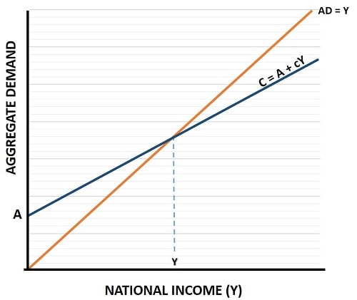
In words this means that consumption (C) is equal to some autonomous spending (A) plus some proportion (c) of national income (Y). We can illustrate this in a graph: 

It's useful to remember that this formula is usually presented to students of economics at a very early stage in their learning, and that it is used to represent spending in an extremely simplified economy where there is no government expenditure and no foreign trade, at least initially.

My main page about the consumption function does explain the concept in more detail and in a more real-world setting that includes government spending, imports & exports, and investment spending. However, it does help to have an article that just focuses on the basics, and that is this purpose of this article.

Explaining the Graph

First of all, consider the AD=Y line. It is drawn with a 45 degree slope indicating that for each extra unit of national income, consumption increases by the same amount. Naturally, consumption does not rise like this in the real world because people will tend to save some part of their increased income for later (or at least run up smaller debts).

For this reason, the slope of the function C = A +cY is less steep than the AD=Y line. It's slope is less than 45 degrees, and is equal to the proportion of income that is spent. A stated above, that proportion (known as the marginal propensity to consume) in represented by the lowercase letter (c) above, and it ranges between zero and one (typically at about 0.6).

Next up, we should note that if national income were to somehow reach zero, consumption would still need to run at some minimum level in order for people to survive. We call this 'autonomous consumption' because it exists autonomously of national income. The implication here is that people will be spending out of their savings or borrowing money to spend.

The consumption function formula illustrated in the graph above shows that spending will be higher than income up until it intersects the AD=Y line, after which national income would be higher than consumption. We can calculate the level of saving in this simplified economy with another function called the saving function.

Consumption Function Formula Example

By plugging some actual numbers into the consumption function formula we can give an example of how to calculate consumption and national income at the equilibrium point in this simplified economy (remember, we assume no government and no foreign trade).

To do this we need to assume a certain amount of investment. Investment in the real world is dependent on many complex factors, and is extremely volatile depending on business confidence levels. However, in this simple model, any investment can only be funded by saving. So investment equals saving.

For the sake of the example, let's just assume investment is $2tn. Let's further assume that that the marginal propensity to consume is 0.6 and that autonomous consumption is $1tn. That gives us:

Y = C + 2

(In words, national income equals consumption plus investment.)

C = 1 + 0.6(Y)

Now, inserting the second equation into the first we get:

Y = 1 + 0.6(Y) + 2

Rearranging for Y we get 0.4(Y) = 3, or Y = 3/0.4 which means Y = $7.5tn. Since national income (Y) is $7.5tn at the equilibrium point, we can deduce from the first equation i.e., Y = C + 2, that consumption must be equal to $5.5tn at the equilibrium point.

This simple example is the sort of elementary consumption function formula problem that you might come across in basic economics.

Related Pages:

• Consumption Function Shifts
• Determinants of Consumption
• The Keynesian Consumption Function

ShareFacebookXPinterestTumblrRedditWhatsApp