The Beveridge Curve (Graphs & Real-World Examples)

Despite having been around for a long time, the Beveridge Curve model of unemployment has received relatively little attention in economic circles, until recently. Research by some of today's leading economists has adapted the theory, with accompanying claims of highly accurate accounting of employment patterns over recent decades.

Whilst the old theory presented a simple downward sloping curve that illustrated the relationship between job vacancy rates and unemployment rates (i.e. when vacancies are high unemployment tends to be low and vice-versa) in an economy, the latest adaptation includes a more sophisticated model of job matching flows into and out of the labor market.

In this report I will give an elementary explanation of the Beveridge curve, and go on to relate it to the main forms of unemployment that exist in the economy (with particular focus on cyclical and structural unemployment).

What is the Beveridge Curve

The Beveridge curve is named after Lord William Henry Beveridge (1879 - 1963), the founder of the modern British welfare system, and whilst he never illustrated his ideas into the standard graph below, he did write extensively on the main ideas behind it.

The Beveridge Curve Graph

Graph of the Beveridge curve showing the inverse relationship between the unemployment rate and the job vacancy rate, with movements along the curve representing economic cycles and shifts indicating changes in labour market efficiency.

The Beveridge curve illustrates the negative relationship between unemployment and job vacancies. Movements along the curve reflect cyclical changes, while shifts signal structural changes in the labour market.

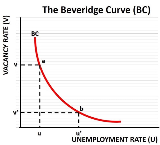
The two basic variables under investigation are the jobs vacancy rate and the unemployment rate. The vacancy rate is usually illustrated on the vertical axis of the Beveridge Curve graph above, whilst the unemployment rate goes on the horizontal axis. The curve, sometimes called the uv curve, illustrates that the relationship between these two variables is a negative one, i.e. as one increases the other decreases.

The simple idea here is that, in times of rapid economic expansions, business will increase the job openings rate as they seek to expand economic production. As a consequence, more people will enter employment and so the unemployment rate will fall. The reverse logic applies in times of recession.

In the graph, we can see that an economy which is at point a is at a higher point in the business cycle than an economy at point b. In other words, movements along the Beveridge curve are associated with changes in cyclical unemployment.

Job Separation and Vacancy Matching

Now, as mentioned above, modern adaptations of the model focus on flows of vacancies and unemployment rather than stocks. These variables are in constant flux and never settled and so the flow concept works better. It also leads us to realize that one of the key metrics to think about is the 'matching' of unemployed people to the existing job opening rate, and the 'separation rate' of workers from their jobs.

The range of factors that can influence the vacancy matching process (i.e. the prevailing rate of unemployment) is extensive, and there has been plenty of research done to try and estimate the most important types that have affected real world unemployment rates over recent decades. The most important of these include:

Wage Rates - since higher wages will encourage workers to accept more jobs.
Generosity of Unemployment Benefits - will discourage workers to accept jobs.
Productivity Growth - will usually increase demand for workers.
The Real Interest Rate of Savings/Assets - increases income from non-work.
Employment Protection Laws - may deter firms from recruiting.
Barriers to Labor Mobility - prevent workers from taking jobs.
Labor Market Policies - may help to increase job take up.
Labor Taxes on employers - make recruitment more expensive.
Labor Taxes on employees - make work less rewarding.
Terms of Trade with foreign countries - increase or decrease demand for workers via changes in demand for domestic goods/services.

The list goes on, but I think you can see that there are lots of factors at play here.

The inclusion of wage rates in the list is a little controversial since it is not independent of the other factors, and will in large part be determined by those other factors in the same way that unemployment is determined by them.

When the separation rate and/or job matching process results in a greater or lesser number of people in employment relative to the number of vacancies that exist, there will be a shift of the Beveridge curve, as discussed below.

Economic lessons from Beveridge Curve shift analysis

With the observed unemployment rates since the 1960s shifting significantly through the 1980s and into the 1990s and beyond, much of the economic research into the Beveridge curve has centered around estimating the influence of the factors listed above. The PDF research papers linked to below will be of interest to anyone who wishes to look into that, but for now I want to illustrate what happens when the separation rate and the vacancy matching rate changes.

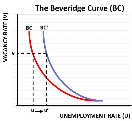
In the graph below I've drawn a Beveridge curve shift from BC to BC'. This sort of shift will occur anytime that people enter unemployment faster, or fill vacancies at a slower rate, due to one 'economic shock' or another. In the 1980s this happened due to the extensive deindustrialization that occurred in many western economies at that time.

A Beveridge Curve Shift

Conceptual illustration of the Beveridge curve showing an outward shift of the curve, indicating reduced labour market matching efficiency between unemployment and job vacancies.

An illustrative shift of the Beveridge curve, where higher unemployment exists alongside more job vacancies, often interpreted as evidence of structural problems in the labor market.

The problem with deindustrialization is that, as manufacturing jobs are lost, even if there is a full compensating effect of growth in service industry jobs (there wasn't full compensation, but lets just suppose so for simplicity) there will be a resulting mismatch between the skills that redundant workers have, and those that employers need. The effect of this is to slowdown the vacancy matching process, causing a rightward shift of the Beveridge curve as shown above.

Starting with an unemployment rate of u and a vacancy rate of v, the original Beveridge curve predicts economic stability given the existing vacancy matching rate. However, after deindustrialization leads to a skills mismatch, a slower matching process results that leads to a new curve at BC'. Given the existing flow of vacancies (which we continue to assume is constant) we reach a new, higher level of unemployment at u'.

Beveridge curve shifts of this sort can be thought of as occurring due to structural unemployment changes, rather than the cyclical changes which are represented as movement along the original BC curve.

Depending on the severity of the structural unemployment and its underlying causes, the higher unemployment may persist for years or even decades. Of course, the severity and duration of the extra unemployment will depend in part on whether or not the government takes appropriate action to influence those factors listed above over which it has control e.g. unemployment benefit generosity, labor taxes, labor market policies and so on.

Labor Market relationship to the NAIRU & Phillips Curve

The value of the Beveridge curve comes from its extra appreciation of the factors that drive both cyclical and structural unemployment. The NAIRU model uses expectations-augmented Phillips curve analysis to focus on the effects on unemployment that result from changes in the business cycle, and on ill-advised short-run government demand-management policies that aim to reduce unemployment without considering the effects on inflation.

The NAIRU actually has very little to say about what determines the long-run rate of unemployment, or natural rate of unemployment, which is where the Beveridge curve has something more to offer.

Conversely, the Beveridge curve has little to say about inflation, or the consequences of short-run interventions in the economy with respect to its impact on prices. In this model we simply assume that the government pursues a policy of low and stable inflation.

Ideally, a single unified model that can account for changes in the different types of unemployment would be available, but at present it is not. Work is underway to try and produce such a model, but right now that is beyond the frontier of current economic knowledge.

Real-World Examples of the Beveridge Curve

United States

The U.S. Beveridge curve is widely tracked using data from the Bureau of Labor Statistics Job Openings and Labor Turnover Survey (JOLTS). It typically shows:

Movement along the curve during normal business cycles: unemployment rises and vacancy rates fall in recessions, and vice versa during expansions.
Outward shifts during the COVID-19 pandemic and after the 2008-09 Great Recession, indicating weaker matching efficiency in the labor market and structural challenges in filling vacancies.

Economists interpret such shifts as evidence that the U.S. labor market was not operating as efficiently as before, due to skills mismatches, sectoral hiring lags, or other frictions during recovery periods.

United Kingdom

The Beveridge curve for the U.K. similarly reflects changes in unemployment and job vacancy rates:

The U.K. curve also slopes downward, indicating the inverse unemployment-vacancy relationship named after economist William Beveridge.
Major labor market changes (such as those driven by Brexit or post-pandemic shifts) can appear as shifts in the curve when structural mismatches between workers and jobs grow.

FAQs

How is the Beveridge curve different from the Phillips curve?

The Beveridge curve shows the relationship between unemployment and job vacancies, while the Phillips curve describes the relationship between unemployment and inflation. The Beveridge curve focuses on labor market matching efficiency, whereas the Phillips curve is concerned with macroeconomic trade-offs between inflation and unemployment. Together, both curves help economists understand labor market tightness and broader economic conditions.

Why can the Beveridge curve shift even when the economy is growing?

The Beveridge curve can shift during economic growth if structural issues reduce matching efficiency between workers and jobs. Skill mismatches, geographic immobility, regulatory changes, or changes in labor force participation can all cause outward shifts in the Beveridge curve, even when GDP is rising and job vacancies are increasing.

What does an inward shift of the Beveridge curve indicate?

An inward shift of the Beveridge curve indicates improved labor market efficiency. This means that for any given unemployment rate, fewer job vacancies are needed to fill open positions. Such shifts may occur due to better job matching technologies, improved education and training, or increased labor market flexibility.

How does automation affect the Beveridge curve?

Automation can influence the Beveridge curve by increasing structural unemployment if workers’ skills do not match new job requirements. This often results in an outward shift of the Beveridge curve, where high vacancy rates coexist with elevated unemployment. Over time, retraining and labor reallocation can partially reverse this effect.

How did the COVID-19 pandemic affect the Beveridge curve?

The COVID-19 pandemic caused sharp movements and outward shifts in the Beveridge curve in many countries. Job vacancies recovered quickly in certain sectors, while unemployment remained elevated due to health concerns, sectoral disruptions, and changes in worker preferences. This highlighted significant matching inefficiencies in post-pandemic labor markets.

Why is the Beveridge curve important for policymakers?

Policymakers use the Beveridge curve to distinguish between cyclical unemployment and structural unemployment. If unemployment rises due to movements along the Beveridge curve, stimulus policies may be effective. If unemployment rises due to an outward shift, structural reforms—such as training programs or labor market deregulation—may be necessary.

Conclusion

The Beveridge curve remains one of the most useful tools for understanding how efficiently a labour market matches workers with available jobs. By examining the relationship between unemployment and job vacancies, the Beveridge curve helps distinguish between cyclical fluctuations and deeper structural problems in the economy.

Real-world examples from the United States and the United Kingdom show that movements along the Beveridge curve typically reflect changes in the business cycle, while shifts in the curve itself often signal lasting changes in labor market dynamics, such as skills mismatches, demographic trends, or institutional constraints.

Sources:

S. Nickell, Et al. - The Beveridge Curve, Unemployment & Wages (PDF)

Related Pages:

About the Author
Steve Bain is an economics writer and analyst with a BSc in Economics and experience in regional economic development for UK local government agencies. He explains economic theory and policy through clear, accessible writing informed by both academic training and real-world work.
Read Steve’s full bio

The Beveridge Curve (Graphs & Real-World Examples)

What is the Beveridge Curve

The Beveridge Curve Graph

Job Separation and Vacancy Matching

Economic lessons from Beveridge Curve shift analysis

A Beveridge Curve Shift

Labor Market relationship to the NAIRU & Phillips Curve

Real-World Examples of the Beveridge Curve

United States

United Kingdom

FAQs

Conclusion

Recent Articles

What Happens to House Prices in a Recession?

Does Government Spending Cause Inflation?

What Happens to Interest Rates During a Recession

Circular Flow Diagram in Economics: How Money Flows

What Happens to House Prices During Stagflation?