- Home
- Aggregate Demand
- Is-lm Model
- IS Curve

The IS Curve Derived & Explained
The IS curve adds more detail to the Keynesian economic model that I have been developing, but to understand it you first need to understand the more basic models on other pages.
In particular I would advise you to start with my page about the Consumption Function before reading this page because you will need the information on that page to make sense of what follows here.
If you already understand the necessary prerequisites, you find that this page is really easy to understand.
Before I get going, keep in mind that the IS curve is a continuation of Keynesian economic theory, and as such the usual assumptions apply i.e. that this is a short-run model of the economy in which production can be increased without any impact on the price level.
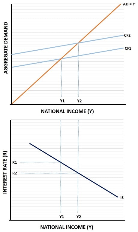
Okay, the diagram below might look a little intimidating to some people but, if you read up on the consumption function as suggested, it will quickly become virtually self-explanatory.

The top half of the diagram should look familiar, it is a simple output expenditure model that shows how an increase in the consumption function leads to an increase in national income/output (with implied increase in employment).
The bottom half of the diagram is the new part that builds new depth to the model.
The IS curve introduces interest rates into the model where previously they had been absent. Investment had been held as one of the autonomous components of aggregate demand that fluctuated according to the level of business confidence, but here we add an extra dimension to show that investment levels are also higher when interest rates are lower.
The downward sloping IS curve illustrates this concept, with the interest rate plotted on the vertical axis against national income/output on the horizontal axis.
The reason why lower interest rates encourage more investment is because business can borrow money more cheaply when interest rates are lower, meaning that more investment projects become viable. In other words, at high interest rates some potential investment projects are ruled out because they are deemed unlikely to make enough profit to cover the expense of borrowing, but as that cost comes down those projects become profitable.
In the diagram, a reduction in the interest rate from R1 to R2 led to a boost in the consumption function from CF1 to CF2, and the economy expanded until a new equilibrium income/output level was achieved at Y2.
From the consumption function, the IS curve has been derived.
The slope of the IS Curve
Adding a little more complexity to the IS curve we can relate it to the Keynesian Multiplier, and as before I recommend that you click the link to get the background information on that concept in order to understand the next diagram.

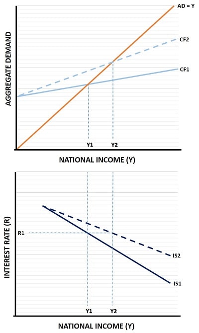
The slope of the IS curve relates to the size of the multiplier. Starting with the top part of the diagram, imagine that for some reason consumer confidence rises in such a way that people start spending more of their money rather than saving it.
This is not uncommon, and sometimes signals the start of a bubble market e.g. in housing.
As people increase their spending, consumption increases and the consumption function gets steeper, as shown by the move from CF1 to the dashed line CF2.
This will cause an increase in national income as firms raise output and employment levels. Gradually, income rises from Y1 to Y2.
Now, since the increase in output was driven by an upturn in consumer confidence that led to an increase in spending (rather than a reduction in the interest rate spurring on extra investment), the interest rate is unchanged in the bottom half of the diagram at R1.
Of course, this sort of extra spending in the economy will lead to extra profits being earned by businesses, which may in turn lead to an increase in business confidence such that investment levels increase at the existing interest rate. This could lead to the same shift in the IS curve that an increase in government spending would cause - see the next diagram for an explanation.
Fiscal Policy and the IS Curve
So far I've focused on explaining the sorts of driving forces in the economy that can lead to movements in the IS curve independently of any sort of government policy aimed at boosting the economy, or slowing it down in times of overheating. However, Keynesian theory is not a dormant inactive doctrine, it is developed with the aim of justifying an active short-term economic policy to try an stabilize the economy in the face of turbulent business/consumption cycles.

You may recall from my pages about the consumption function that government spending is one of the autonomous components of aggregate demand, and that it can be used to boost the economy in times when this is deemed necessary.
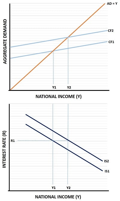
In this diagram, we can see how the effects of a discretionary fiscal stimulus will affect the economy.
Starting with the top half of the diagram, an increase in government spending causes the CF1 line to rise to CF2. The extra spending in the economy offsets whatever loss of spending caused a downturn in the economy (for the purposes of this section, imaging that at an output/income level of Y1 the economy is under-performing).
The extra spending caused by the fiscal stimulus restores profitability in the business sector and supports an increase in production such that income/output increases to its desired level at Y2.
In the bottom half of the diagram you can see that, with interest rates unaltered, the entire IS curve has shifted to the right to reflect the new equilibrium point in the goods market.
This is one of the main points to keep in mind, fiscal policy works by causing a shift in the IS curve. This does not mean that only fiscal policy can cause such shifts, far from it, but in most of the Keynesian models that you will come across, shifts in the IS curve are usually attributed to fiscal policy.
Summary of Main Points
- A change in the interest rate will cause changes in the pattern of consumption levels and this will affect the level of national income and output. This will cause a movement along the existing IS curve to reflect the new interest rate and the new level of income.
- A change in the factors that determine the multiplier will cause a change in the slope of the consumption function and, in turn, a change in the slope of the IS curve. The new curve will reflect a new income output level at the existing interest rate.
- A change in any of the autonomous components of aggregate demand will cause a shift in the entire consumption function as well as a shift in the entire IS curve. Interest rates are again unaltered by such changes in autonomous spending.
Criticisms
I won't go too deeply into my main criticisms of the IS curve on this pages because it is better to put my main objections altogether in one place, and the best place for that is on my page about the full IS-LM Model.
However, I think you will already appreciate the complexity of the Keynesian model that we are dealing with here and the near impossibility of deriving accurate policy initiatives from it in a timely manner.
The diagrams above are all well and good from an analysis point of view but just take a moment to consider all the ramifications in the real world that affect these variables in completely unpredictable ways. The economy doesn't simply standstill and wait for policy makers to react to the events of the day, those events are constantly evolving.
We do not know, for example, where any of theses curves actually sit at the current time. We do not know how they are moving, and we don't even know in which direction they are headed. All we have is out-of-date information that suggests where the curves might have been in a prior period.
Now imagine how difficult it would be to put together a sensible set of policies to move these curves in the desired direction, knowing full well that by the time they take effect the already out -of-date picture of the economy that we have will be even more obsolete.
This is all before we have to deal with the political influences that often lead to inappropriate economic policies for vote-maximizing purposes...
I mean, can anyone in their right mind look at the budget deficit, the national debt, the low-growth, the crony capitalism, and so on ad-infinitum and believe that governments are capable of sensible macroeconomic management of our economies - because I'm not seeing it?
Related Pages:
- The Consumption Function
- Autonomous Consumption
- The Keynesian Multiplier
- Aggregate Demand
- The LM Curve
- The IS-LM Model
- Real Balance Effect
- Cyclical Unemployment
About the Author
Steve Bain is an economics writer and analyst with a BSc in Economics and experience in regional economic development for UK local government agencies. He explains economic theory and policy through clear, accessible writing informed by both academic training and real-world work.
Read Steve’s full bio
Recent Articles
-
Bank Reserves, Asset Inflation, and the Risk of Future Price Inflation
Dec 19, 25 04:16 AM
Learn what bank reserves are, how they affect asset prices, and why future reserve creation could lead to inflation through commodities and currencies. -
Credit Creation Theory; How Money Is Actually Created
Dec 16, 25 03:07 PM
Explore how modern banks create money through credit creation, why the money multiplier fails, and the role of central banks and reserves. -
U.S. Industrial Policy & The Unfortunate Sacrifice that Must be Made
Dec 12, 25 03:03 AM
U.S. Industrial Policy now demands a costly tradeoff, forcing America to rebuild its industry while sacrificing bond values, pensions, and the cost of living. -
The Global Currency Reset and the End of Monetary Illusion
Dec 07, 25 03:48 AM
The global currency reset is coming. Learn why debt, inflation, and history’s warnings point to a looming transformation of the world’s financial system. -
Energy Economics and the Slow Unraveling of the Modern West
Dec 06, 25 05:18 AM
Energy economics is reshaping global power as the West faces decline. Explore how energy, geopolitics, and resource realities drive the unfolding crisis.